How do we know that the CMB is from a hot, early Universe?

Towards the end of July I had an article published in The Conversation about the Cosmic Microwave Background, follow this link to read that article. After the article had been up a few days, I got this question from a Mark Robson, which I thought was an interesting one.

Mark Robson’s original question which be posed below the article I wrote for The Conversation.

I decided to blog an answer to this question, so the blogpost “What is the redshift of the Cosmic Microwave Background (CMB)?” appeared on my blog on the 30th of August, here is a link to that blogpost. However, it would seem that Mark Robson was not happy with my answer, and commented that I had not answered his actual question. So, here is his re-statement of his original question, except to my mind he has re-stated it differently (I guess to clarify what he actually meant in his first question). 

I said I would answer this slightly different/clarified question soon, but unfortunately I have not got around to doing so until today due to various other, more pressing, issues (such as attending a conference last week; and also writing articles for an upcoming book 30-second Einstein, which Ivy Press will be publishing next year).

The questions and comments that Mark Robson has since posted below my article about how we know the redshift of the CMB

What is unique about the CMB data?

The very quick answer to Mark Robson’s re-stated question is that “the unique data possessed by the CMB which allow us to calculate its age or the temperature at which it was emitted” is that it is a perfect blackbody. I think I have already stated in other blogs, but let me just re-state it here again, the spectrum as measured by the COBE instrument FIRAS in 1990 of the CMB’s spectrum showed it to be the most perfect blackbody spectrum ever seen in nature. Here is the FIRAS spectrum of the CMB to re-emphasise that.

The spectrum of the CMB as measured by the FIRAS instrument on COBE in 1990. It is the most perfect blackbody spectrum in nature ever observed. The error bars are four hundred times larger than normal, just so one can see them!

So, we know, without any shadow of doubt, that this spectrum is NOT due to e.g. distant galaxies. Let me explain why we know this.

The spectra of galaxies

If we look at the spectrum of a nearby galaxy like Messier 31 (the Andromeda galaxy), we see something which is not a blackbody. Here is what the spectrum of M31 looks like.

The spectrum of our nearest large galaxy, Messier 31

The spectrum differs from a blackbody spectrum for two reasons. First of all, it is much broader than a blackbody spectrum, and this is easy to explain. When we look at the light from M31 we are seeing the integrated light from many hundreds of millions of stars, and those stars have different temperatures. So, we are seeing the superposition of many different blackbody spectra, so this broadens the observed spectrum.

Secondly, you notice that there are lots of dips in the spectrum. These are absorption lines, and are produced by the light from the surfaces of the stars in M31 passing through the thinner gases in the atmospheres of the stars. We see the same thing in the spectrum of the Sun (Josef von Fraunhofer was the first person to notice this in 1814/15). These absorption lines were actually noticed in the spectra of galaxies long before we knew they were galaxies, and were one of the indirect pieces of evidence used to argue that the “spiral nebulae” (as they were then called) were not disks of gas rotating around a newly formed star (as some argued), but were in fact galaxies outside of our own Galaxy. Spectra of gaseous regions (like the Orion nebula) were already known to be emission spectra, but the spectra of spiral nebulae were continuum spectra with absorption lines superimposed, a sure indicator that they were from stars, but stars too far away to be seen individually because they lay outside of our Galaxy.

The absorption lines, as well as giving us a hint many years ago that we were seeing the superposition of many many stars in the spectra of spiral neublae, are also very useful because they allow us to determine the redshift of galaxies. We are able to identify many of the absorption lines and hence work out by how much they are shifted – here is an example of an actual spectrum of a very distant galaxy at a redshift of , and below the actual spectrum (the smear of dark light at the top) is the identification of the lines seen in that spectrum at their rest wavelengths.

The spectrum of a galaxy at a redshift of z=5.515 (top) (z=5.515 is a very distant galaxy), and the features in that spectrum at their rest wavelengths

Some galaxies show emission spectra, in particular from the light at the centre, we call these type of galaxies active galactic nucleui (AGNs), and quasars are now known to be a particular class of AGNs along with Seyfert galaxies and BL Lac galaxies. These AGNs also have spectral lines (but this time in emission) which allow us to determine the redshift of the host galaxy; this is how we are able to determine the redshifts of quasars.

Notice, there are no absorption lines or emission lines in the spectrum of the CMB. Not only is it a perfect blackbody spectrum, which shows beyond any doubt that it is produced by something at one particular temperature, but the absence of absorption or emission lines in the CMB also tells us that it does not come from galaxies.

The extra-galactic background light

We have also, over the last few decades, determined the components of what is known as the extra-galactic background light, which just means the light coming from beyond our galaxy. When I say “light”, I don’t just mean visible light, but light from across the electromagnetic spectrum from gamma rays all the way down to radio waves. Here are the actual data of the extra-galactic background light (EGBL)

Actual measurements of the extra-galactic background light

Here is a cartoon (from Andrew Jaffe) which shows the various components of the EGBL.

The components of the extra-galactic background light

I won’t go through every component of this plot, but the UV, optical and CIB (Cosmic Infrared Background) are all from stars (hot, medium and cooler stars); but notice they are not blackbody in shape, they are broadened because they are the integrated light from many billions of stars at different temperatures. The CMB is a perfect blackbody, and notice that it is the largest component in the plot (the y-axis is what is called , which means that the vertical position of any point on the plot is an indicator of the energy in the photons at that wavelength (or frequency). The energy of the photons from the CMB is greater than the energy of photons coming from all stars in all the galaxies in the Universe; even though each photon in the CMB carries very little energy (because they have such a long wavelength or low frequency).

Why are there no absorption lines in the CMB?

If the CMB comes from the early Universe, then its light has to travel through intervening material like galaxies, gas between galaxies and clusters of galaxies. You might be wondering why we don’t see any absorption lines in the CMB’s spectrum in the same way that we do in the light coming from the surfaces of stars.

The answer is simple, the photons in the CMB do not have enough energy to excite any electrons in any hydrogen or helium atoms (which is what 99% of the Universe is), and so no absorption lines are produced. However, the photons are able to excite very low energy rotational states in the Cyanogen molecule, and in fact this was first noticed in the 1940s long before it was realised what was causing it.

Also, the CMB is affected as it passes through intervening clusters of galaxies towards us. The gas between galaxies in clusters is hot, at millions of Kelvin, and hence is ionised. The free electrons actually give energy to the photons from the CMB via a process known as inverse Compton scattering, and we are able to measure this small energy boost in the photons of the CMB as they pass through clusters. The effect is known as the Sunyaev Zel’dovich effect, named after the two Russian physicists who first predicted it in the 1960s. We not only see the SZ effect where we know there are clusters, but we have also recently discovered previously unknown clusters because of the SZ effect!

I am not sure if I have answered Mark Robson’s question(s) to his satisfaction. Somehow I suspect that if I haven’t he will let me know!

Read Full Post »

Emission Line Spectra

I have referred a few times to line spectra. In my blog about the Messier catalogue, I mentioned that M42 and M1 were both examples of objects which exhibited an emission line spectrum. And in my blog on the three kinds of spectra, of course emission line spectra are one of the three types. So, how do emission line spectra come about?

Electrons in orbit about the nucleus

In a future blog I will explain in more detail why electrons orbit the nucleus of atoms in only certain allowed energy levels. This was first proposed by Niels Bohr in 1913, and the details were then worked out until a full explanation was developed by Erwin Schrödinger, Werner Heisenberg and Paul Dirac in 1926-1928 in what we now call Quantum Mechanics.

As I mentioned in my blog on the different types of spectra, it was noticed by Kirchhoff and Bunsen in the 1850s that different salts produced different types of line spectra when they were burnt in a flame. This is because each element has an unique spectral signature. We will look at the simplest spectrum, that of the hydrogen atom. It is the easiest to understand, because the hydrogen atom only has one electron. Additional electrons complicate matters, because the electrons interact with each other in their orbits, but for hydrogen things are nice and simple.

The emission line spectrum of hydrogen

Because hydrogen is the simplest element, it is the most abundant in the Universe. About 75% of the “normal” matter in the Universe is in the form of hydrogen. In the visible part of the spectrum, the hydrogen emission line spectrum looks like this.

Notice that there are a series of lines over towards the blue (left) end of the spectrum, and a prominent line in the red, which has an arrow pointing towards it. This line is so common and important in astronomy that it even has a special name, it is called the h-alpha (hydrogen alpha) line.

How do these lines come about?

The explanation for these different lines is that the different lines are produced by electrons jumping down between different energy levels in the hydrogen atom. The electron wants to be in the ground state, the n=1 level, in hydrogen. But it can be excited into higher levels, either by absorbing a photon (a particle of light), or by another electron hitting it. Once it finds itself in a higher energy level (n=2 or higher), it wants to jump back down to the n=1 level as quickly as it can. It is in jumping back down that the photons which we see in an emission line spectrum are produced.

The figure below shows the simplified energy level diagram for hydrogen, with the n=1, n=2, n=3 etc. energy levels. The Balmer series, which are all in the visible part of the spectrum, are produced when electrons jump from a higher energy level into the n=2 level. So e.g. from n=3 to n=2, or n=4 to n=2, or n=5 to n=2. It is the Balmer spectral lines which are shown in the figure above of a hydrogen emission spectrum.

The figure also shows three other “series”, the Lyman series which are in the ultraviolet part of the spectrum, and the Paschen and Brackett series, which are in the infrared part of the spectrum. The Lyman series all end in the n=1 level (ground state), the Paschen series all end in the n=3 level, and the Brackett series all end in the n=4 level.

The energies of the different energy levels in hydrogen

These visible-light lines were well measured in the 1880s, and are referred to as the Balmer series. Balmer had even derived an empirical formula for the wavelengths. He did not know about energy levels, but by slightly adapting his formula we can write an empirical formula for the energy levels of a hydrogen atom [empirical means it was derived through trial and error, with no physical explanation for why the formula works]. It is

This formula gives the energy in eVs, and these values are over on the right of the diagram for each energy level [Note: Chemists will often label the n=1 level as -13.6eV, and work upwards from this, physicists tend to label it as 0eV. It doesn’t matter, because all that is important is the energy difference between different levels]. eV stands for “electron volt”, and is just a more convenient unit for measuring the small energies involved than using the more usual Joules. It’s just like using nanometres to measure things on the atomic scale because metres are too big.
An electron volt is defined as , so is pretty small as you can see.

There is a very simple relationship between the difference in energy between two energy levels and the wavelength of the photon produced when the electron jumps down. The energy of the photon is given by , where is called Planck’s constant and is the frequency of the photon. If you prefer to think in terms of wavelength instead of frequency they are very simply related; the wavelength is just given by where is the speed of light. So, putting this together, we can write that the wavelength of a photon is given by

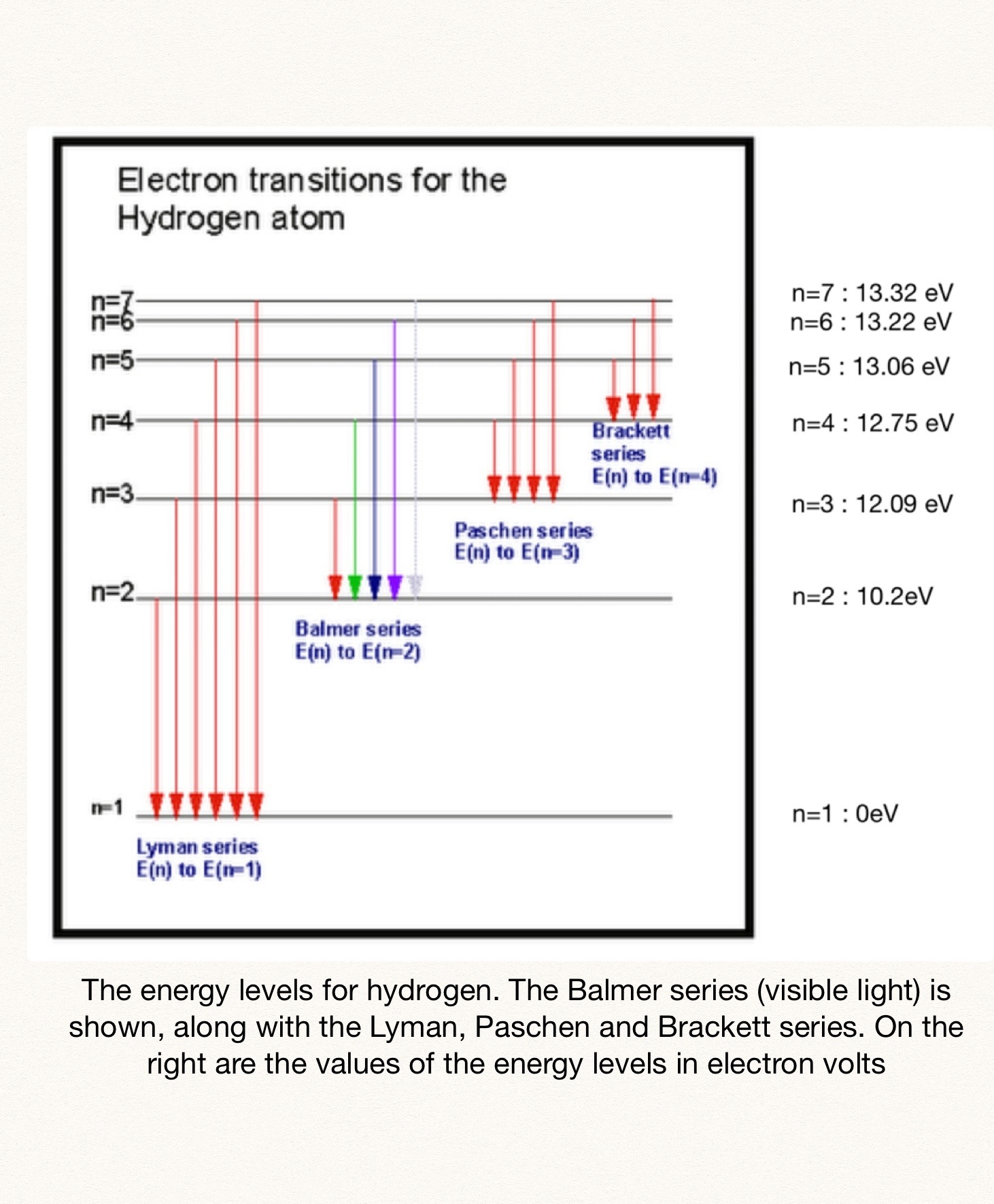
where is the energy difference between the two levels the electron jumps between. To go through a couple of examples, if an electron jumps from the n=3 to the n=2 level, the energy difference is . We need to convert this to Joules, so . To get the wavelength from this we write . This is in the red part of the visible spectrum, and is the hydrogen-alpha line we were referring to earlier.

To work through a second example, if we look at the transition between n=5 and n=3 (part of the Paschen series) we get . So the photon will have a wavelength of , which is in the infra-red part of the spectrum.

What is true for hydrogen is also true for the other elements, it is just that there is no simple formula for working out the energies of the different energy levels like there is for the energy levels in hydrogen. But, as we shall see in another future blog, even the n=2 and n=3 levels in hydrogen are not all at exactly the same level, it depends on the angular momentum of the electron in a particular energy level. This is where the s,p,d,f lines that I mentioned in this blog comes into play. So what I have explained above is a first approximation, but perfectly fine for most uses.

Read Full Post »